Venus Volcanoes Data Analysis
Welcome to the Data Analysis section of the project.
In this section, we spend most of the time on
Data Cleansing
Data Exploration
Data Preparation
These are the crucial steps for any machine learning project as hygiene data yields robust models.
In this section, I have used the following python libraries:
Numpy
Pandas
Matplotlib
Pylab
Data Exploration
Dimensions of Dataset:
## Training Data: (7000, 12100)## Testing Data: (2734, 12100)Sample of DataFrame
##      0    1    2    3   4    5  ...  12095  12096  12097  12098  12099  Volcano
## 0   95  101   99  103  95   86  ...     99    117    116    118     96        1
## 1   91   92   91   89  92   93  ...    105    104    100     90     81        0
## 2   87   70   72   74  84   78  ...     80     91     80     84     90        0
## 3    0    0    0    0   0    0  ...     90     92     80     88     96        0
## 4  114  118  124  119  95  118  ...    104    106    117    111    115        0
##
## [5 rows x 12101 columns]
Corrupted Images
The data that we are dealing with is image data. So, there is a good chance for data corruption.
It seems (also mentioned in data dictionary) that few records are corrupted. Take a look at the fourth record (index = 3) in the above sample dataframe. The record seems corrupted because it is having a bunch of 0’s for the pixel values.
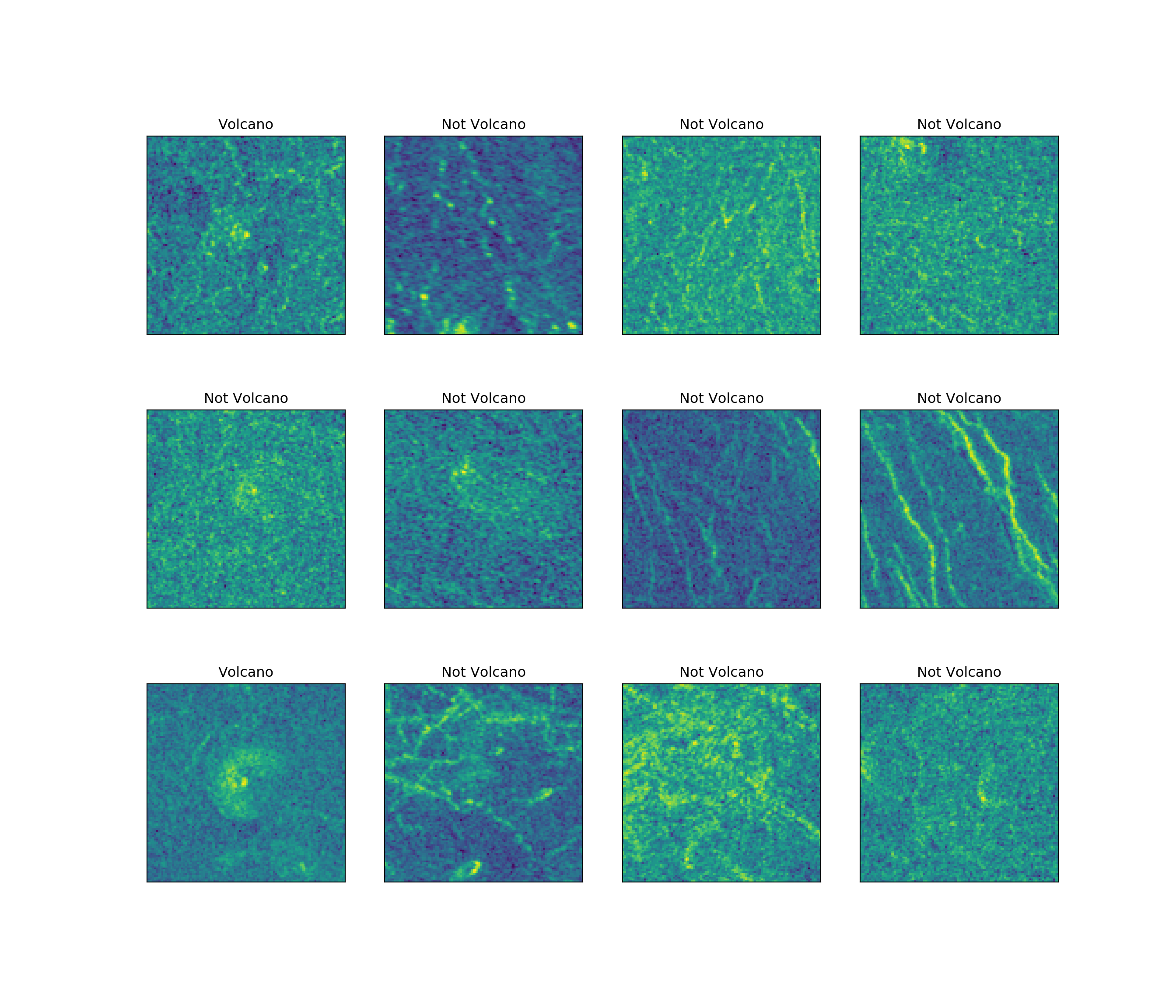
Let’s plot and see a few records and then we will build a work around to find and filter the corrupted records.
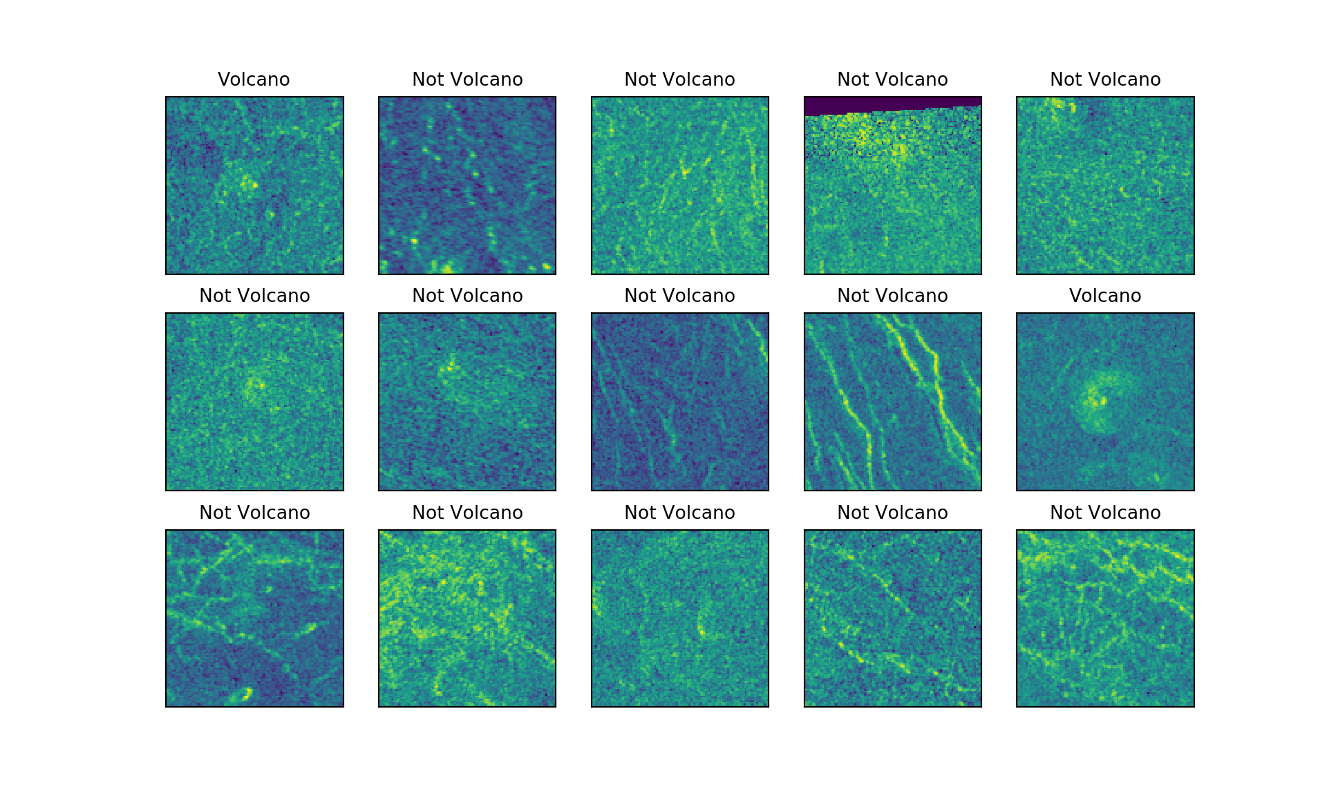
Observations:
- The fourth record has some data corrupted at the top of the image.
Pixel Values Distribution
Let’s look at the pixel value distributions for these images.
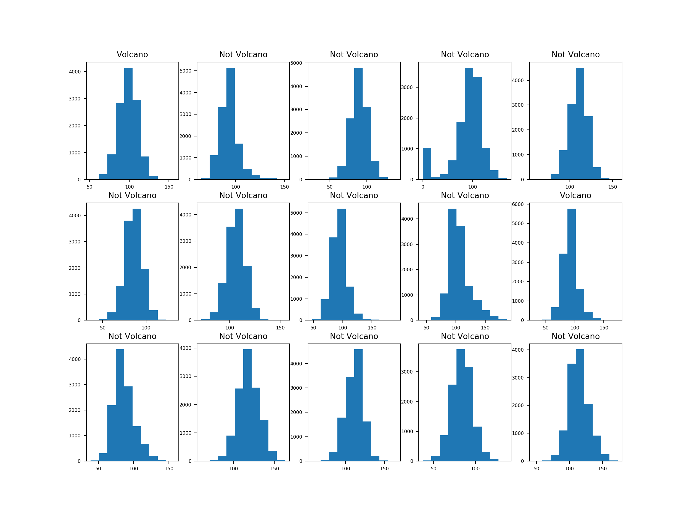
Observations:
- According to the histograms, for the corrupted image (fourth), the number of pixels whose value is 0 are relatively high.
Analyzing Corrupted Pixels
First, let’s calculate the number of Corrupted pixels (pixel value = 0) per image.
Then we will define a threshold to find and filter corrupted records.
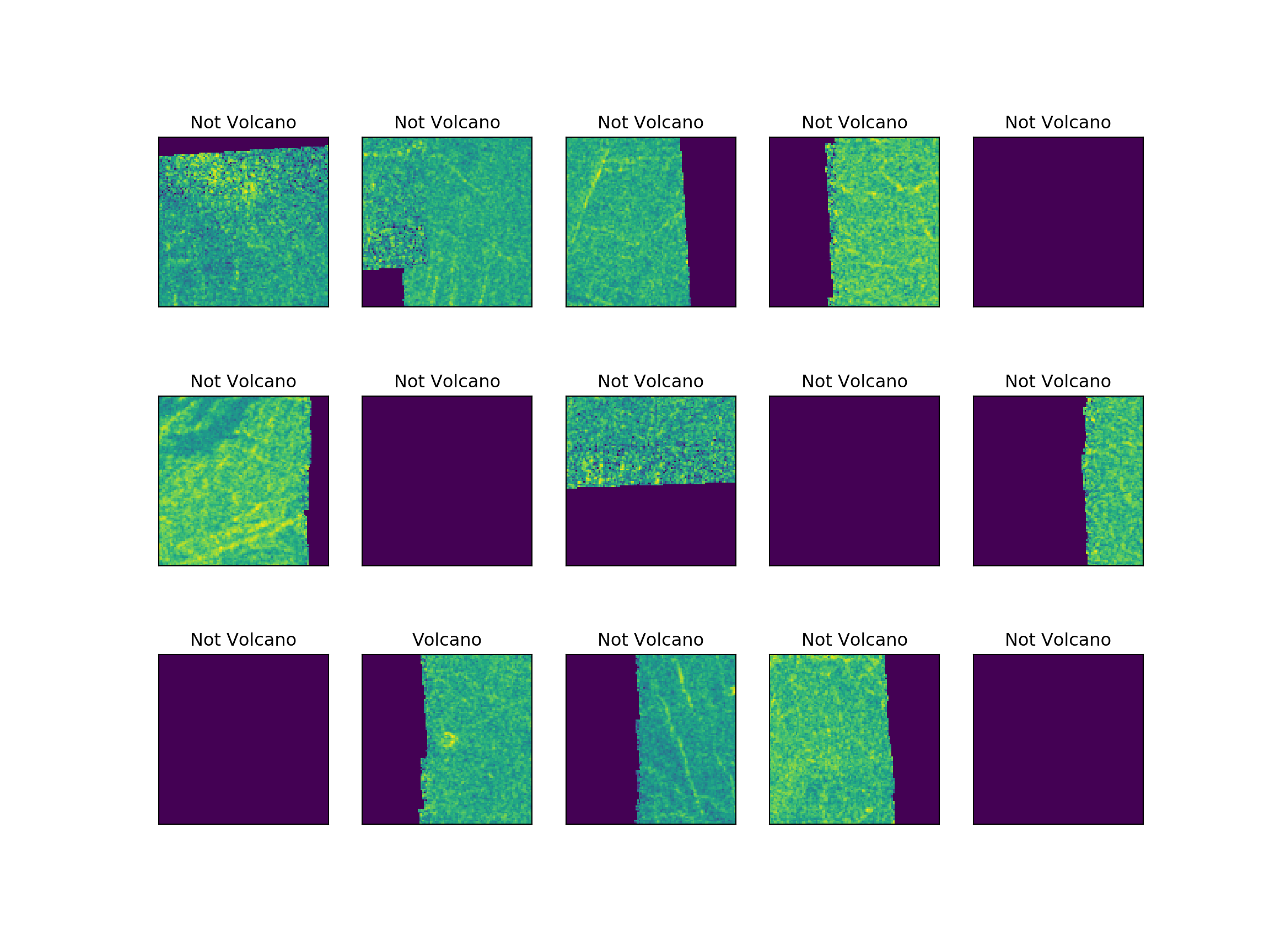
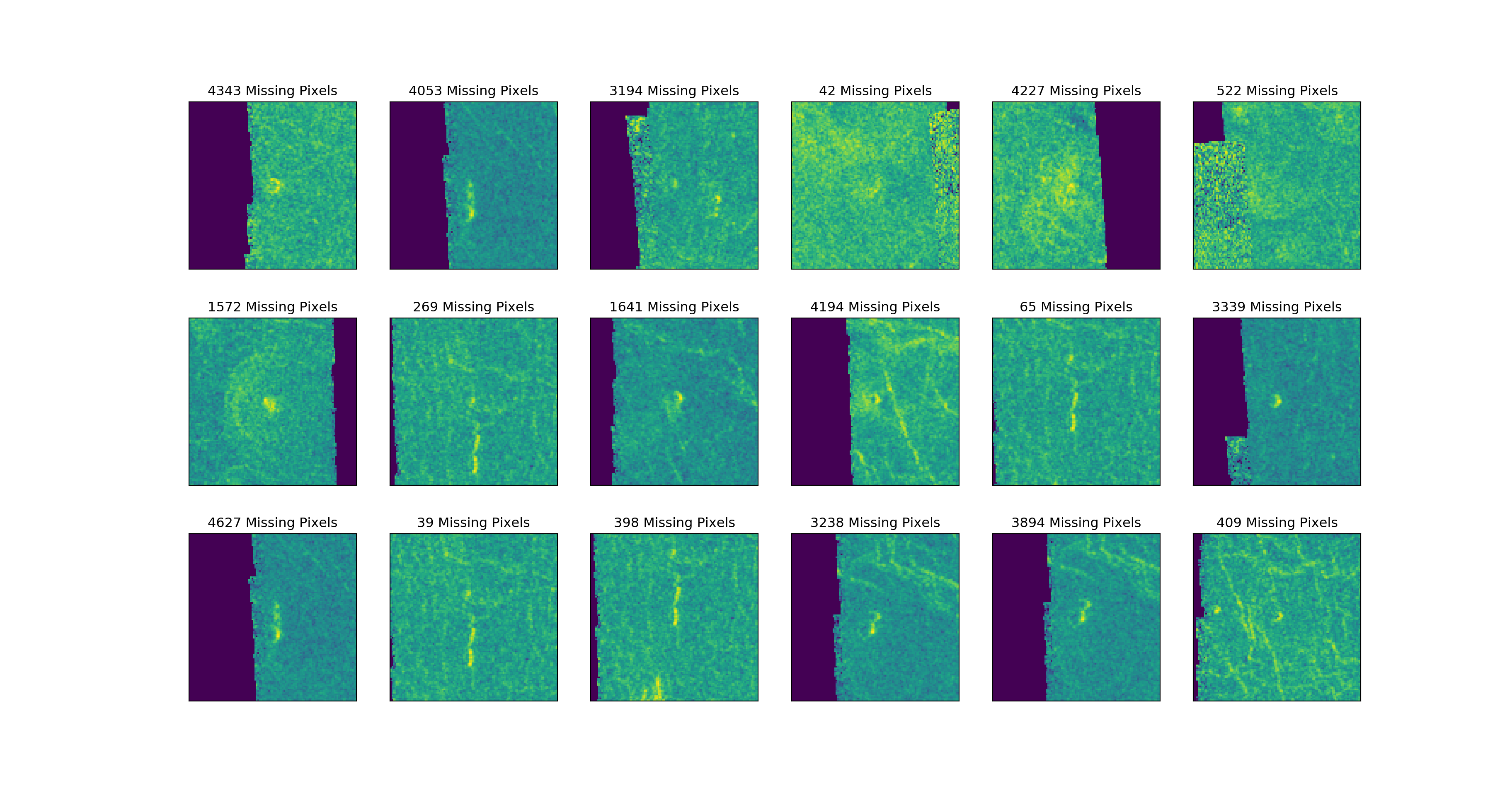
Let’s look at some of the corrupted images
Statistics and Distribution of Corrupted Pixels
## MEAN of Corrupted Pixels 8190.0
##
## STD of Corrupted Pixels 4500.0
##
## MIN of Corrupted Pixels 1.0
##
## 25% of Corrupted Pixels 4020.0
##
## 50% of Corrupted Pixels 11198.0
##
## 75% of Corrupted Pixels 12100.0
##
## MAX of Corrupted Pixels 12100.0
Quartile Plot
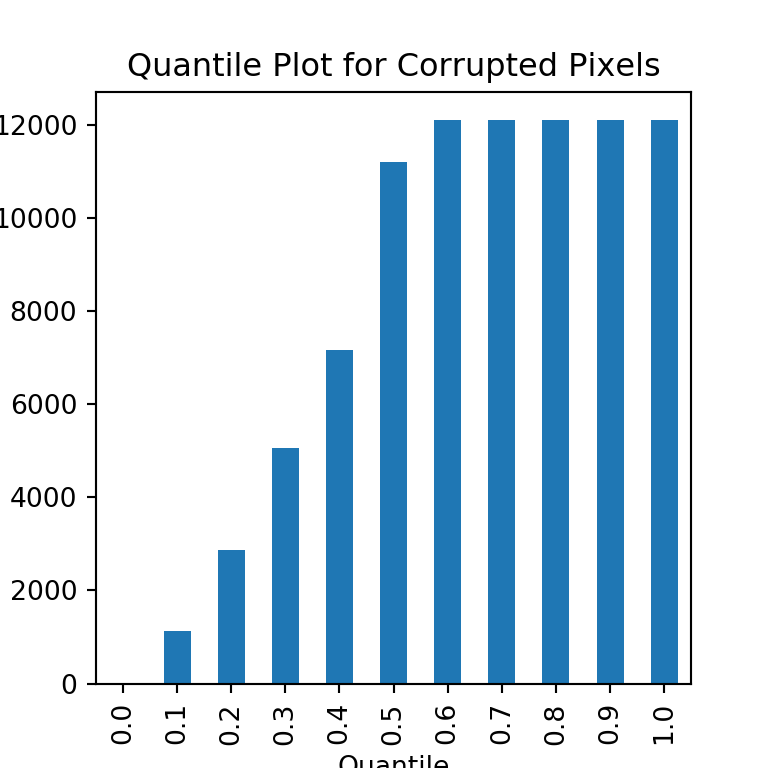
Observations:
Almost 50% of the corrupted images have all the pixels corrupted.
25% of the corrupted images have around 4000 pixels corrupted.
10% of the corrupted images have around 2000 pixels corrupted.
Corrupted Pixels Distribution
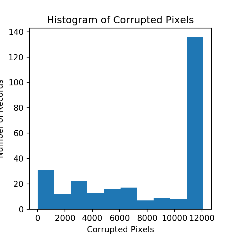
Observations:
- According to the histogram, most of the corrupted images have lot of corrupted pixels.
Let’s pick an example from each bin and see how the image looks

Target Classes in Corrupted Images
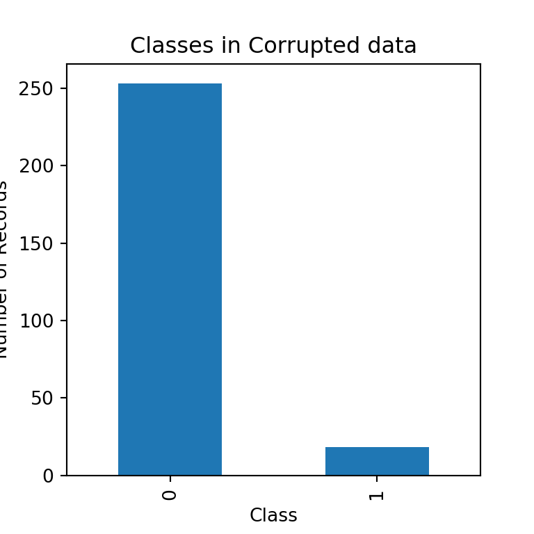
Observations:
Lot of corrupted images do not have volcanoes in them.
Only a few corrupted records do have volcanoes.
Omitting Corrupted Images without Volcanoes
- As our dataset already have a good number of examples without volcanoes, I think it would not be good idea to invest time to define threshold level for missing pixels or to impute data for corrupted pixels that have Volcanoes and omit the records that are corrupted and do not have volcanoes.
Corrupted Images with Volcanoes
Imputing
As we already have a Class Imbalance (very few images with Volcanoes) in the target variable on our original dataset, let’s try not to remove the corrupted images that has volcanoes. Instead, let’s fill the corrupted pixels in the image with the mean values of the image.
But, should we use Row means or Column means?: It seems, for most of the images, the entire column is corrupted. So, let’s use row means of image to replace the corrupted pixel.
Imputing Corrupted Pixels with Row Means
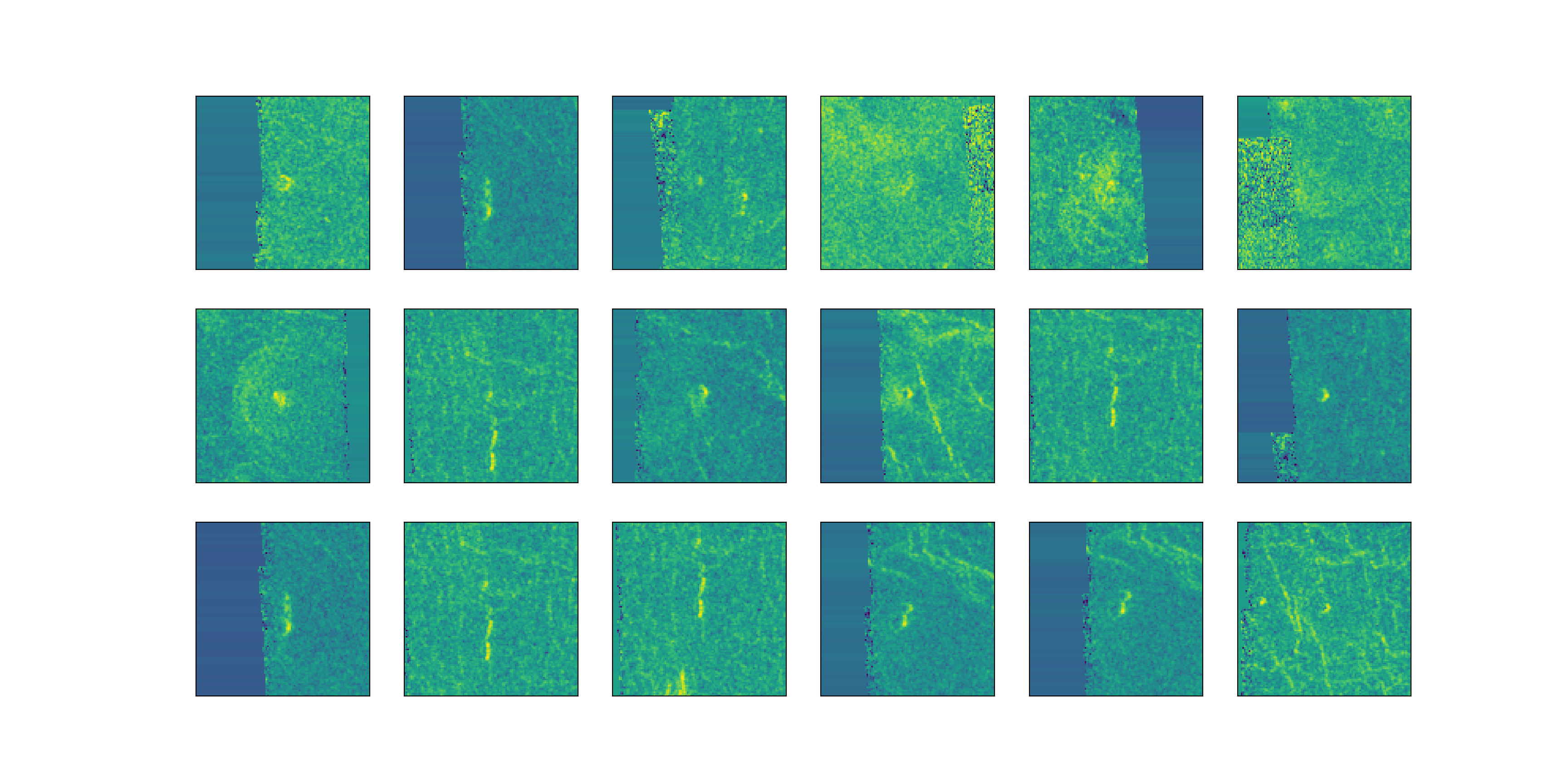
The images doesn’t look good. Row means doesn’t seem like a great idea.
Instead let’s compute the mean of every pixel for all the images that are not corrupted and use those means to replace the corrupted pixels in corrupted images.
Imputing Corrupted Pixels with Pixel Means from all images
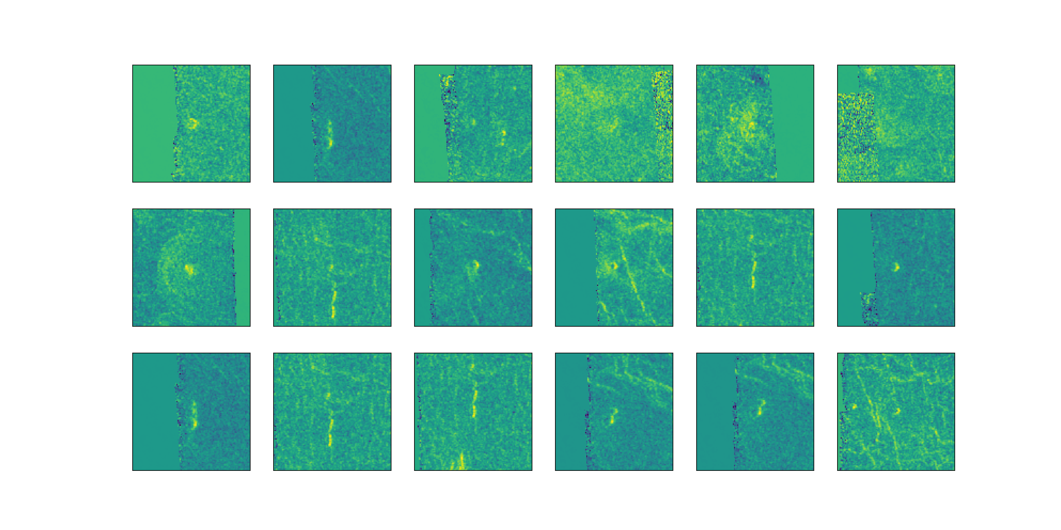
Definitely not a wonderful improvement, but much better than using row means.
Now, in this final attempt, let’s try to replace the missing/corrupted pixels by flipping the image (mirroring) and use the corresponding pixels from flipped image.
Imputing Corrupted Pixels with Pixels from flipped Image
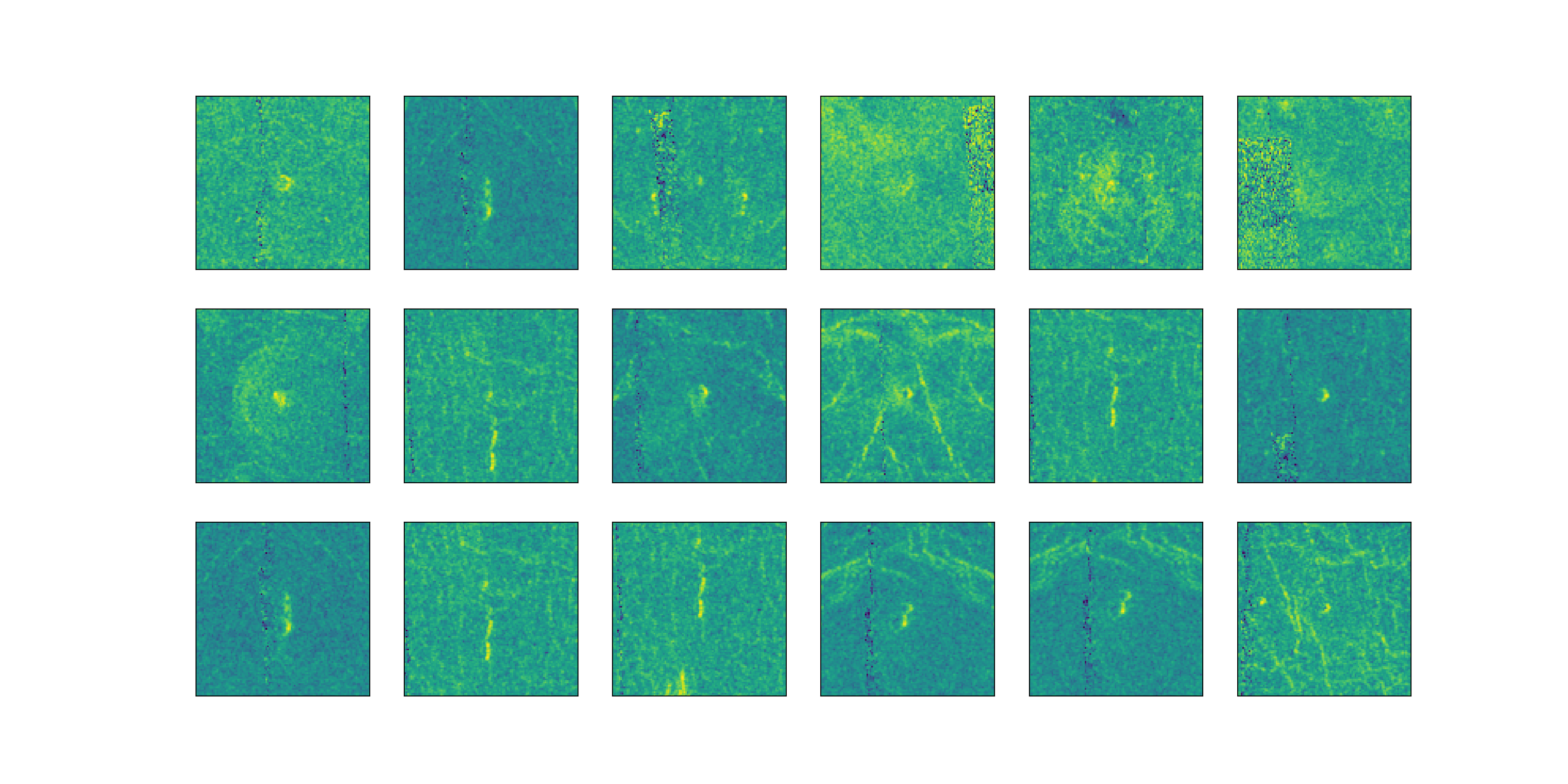
- Awesome, this looks much better than the above two methods. Let’s stick with this!
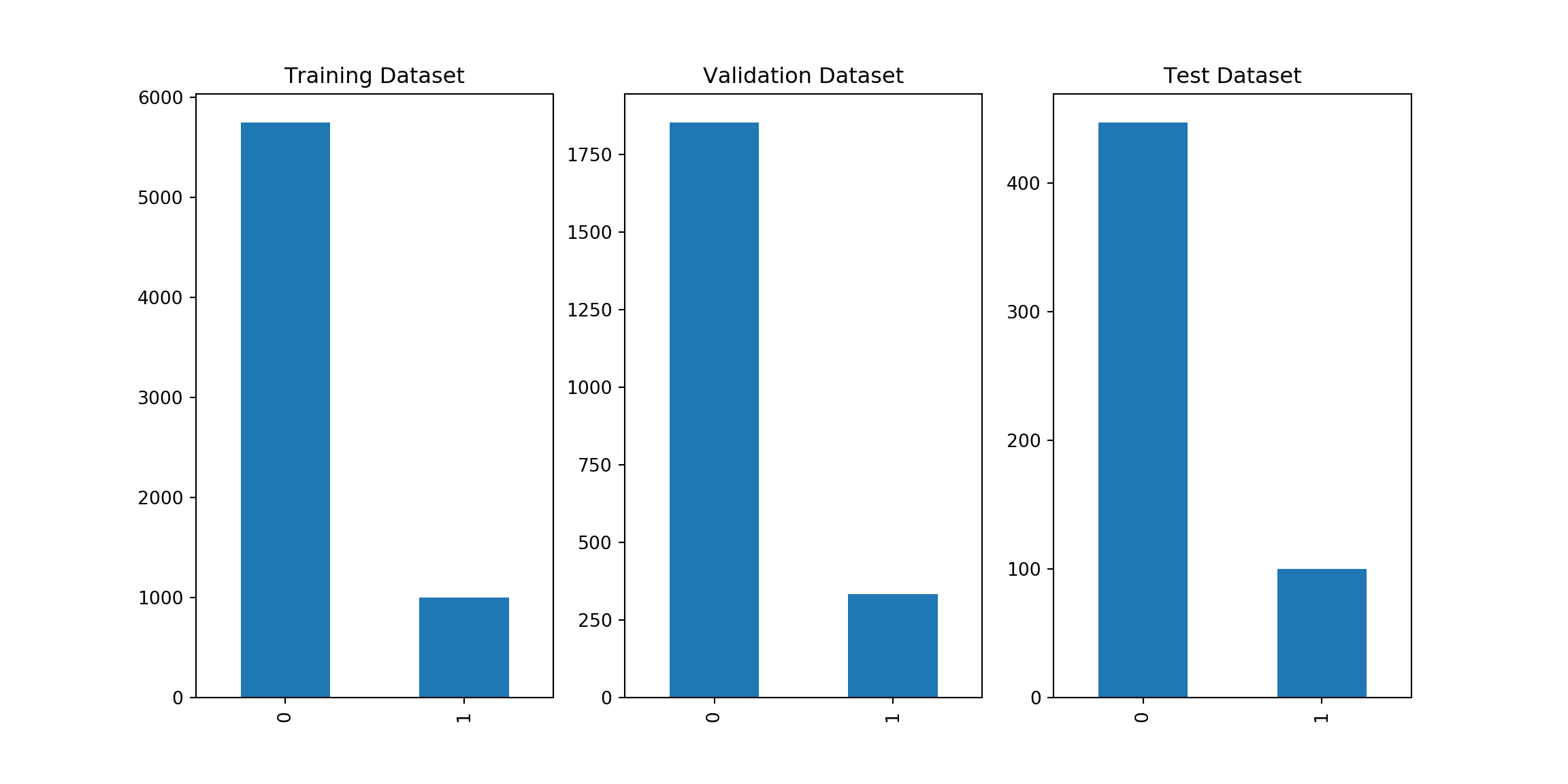
Data Preparation
Creating Train, Validation and Test sets
## Training Samples: 6747## Validation Samples: 2187## Test Samples: 547Target Classes
Normalize
It is a good practice to normalize data before feeding it to the learning algorithm. Algorithms like gradient decent will converge faster if we normalize/standardize the input data.
Sanity Checks
## Number of Input Examples: 6747## Number of Input Features: 12100## X_train shape: (6747, 12100)## y_train shape: (6747,)## X_val shape: (2187, 12100)## y_val shape: (2187, 1)## X_test shape: (547, 12100)## y_test shape: (547, 1)